Your first discovery with pysubgroup
We will ask: which groups in the Adult census-income dataset have a higher
share of the >50K income label than the dataset overall? We describe groups
through attributes such as age, education, occupation, and working hours.
This example demonstrates the discovery workflow on historical records; its
patterns describe associations rather than effects of changing an attribute.
Installation
Use Python 3.11–3.14 in a virtual environment. The package requires NumPy 2 or newer, pandas, SciPy, and scikit-learn. The plotting extra supplies matplotlib:
pip install "pysubgroup[plot]"For a local source checkout, run pip install -e ".[plot]" from the repository
root in your chosen environment. Optional acceleration is introduced in
Making searches practical.
1. Data and a fitted target
Load Adult with scikit-learn’s OpenML loader. The first run requires an internet
connection; subsequent runs reuse the downloaded data. When run from the book
folder, data_home=Path("data-cache") keeps that cache inside user_guide/.
We take a reproducible 3,000-row sample to keep the introductory search small.
from pathlib import Path
from sklearn.datasets import fetch_openml
import pysubgroup as sd

adult = fetch_openml("adult", version=2, as_frame=True, data_home=Path("data-cache"))
columns = ["age", "workclass", "education", "marital-status", "occupation", "sex", "hours-per-week", "class"]
data = adult.frame[columns].sample(n=3000, random_state=42).copy()
X = data.drop(columns="class")
target = sd.BinaryTarget().fit(data, "class", ">50K")
print(f"Rows: {len(data)}; >50K rows: {target.n_positives_}")
print(f"Dataset >50K share: {target.n_positives_ / len(data):.1%}")
data.head()
Rows: 3000; >50K rows: 729
Dataset >50K share: 24.3%
BinaryTarget turns membership in label ">50K" into positive/negative
information for each row. It does not train a classifier. The fitted target
retains the reference statistics needed by quality functions; the printed
dataset share is the baseline against which subgroups will be compared.
The selected columns exclude the census sampling weight fnlwgt, which is not
a descriptor of a person. Here each record counts equally; the example is not
a survey-weighted population estimate. We also retain education rather than
its closely related numeric encoding education-num.
2. Candidate descriptions
conditions = sd.generate_conditions(X, n_bins=4, numeric_candidates="thresholds")
print(f"Candidate conditions: {len(conditions)}")
print("First six conditions (preview, not the complete search space):")
print(*map(str, conditions[:6]), sep="\n")
Candidate conditions: 60
First six conditions (preview, not the complete search space):
age ≤ 33
age > 33
age ≤ 50
age > 50
age ≤ 67
age > 67
Only descriptor attributes enter X; the income label class stays out of the
descriptions. Categorical attributes generate tests such as
education=Bachelors. Numeric attributes provide thresholds such as age ≤ ...
and their > counterparts. n_bins controls discretization, not the maximum
number of conditions in a rule. Missing descriptor values can be matched by an
explicit is_missing condition.
3. Quality, constraints, and search
task = sd.SubgroupDiscoveryTask(
    data=data,
    target=target,
    search_space=conditions,
    qf=sd.WRAccQF(),
    result_set_size=5,
    depth=2,
    min_quality=0,
    filters=[sd.MinSizeFilter(100)],
)
results = sd.DFS().execute(task)
table = sd.to_dataframe(results, data, target)
tableThe task asks for up to five descriptions, each with at most two conditions and
at least one hundred rows. DFS exhaustively searches this permitted space and uses
optimistic estimates to prune branches. Results are (quality, Rule) pairs in
decreasing quality order. With min_quality=0, reported scores must be positive.
Read a row of the table in this order:
Description: which attribute values define membership?
Size: how many records support the finding?
Target share: what fraction of the group has the
>50Klabel?Quality: how does the chosen size–deviation trade-off rank the finding?
A high target share in a large subgroup is rewarded by WRAcc. Several top descriptions may be variations on the same pattern.
4. Inspect actual members
quality, rule = results[0]
members = sd.subgroup_data(rule, data)
print(rule)
print(f"WRAcc: {quality:.4f}; rows: {len(members)}")
members.head()
[age ≤ 67 ∧ marital-status=Married-civ-spouse]
WRAcc: 0.1005; rows: 1323
Inspecting rows is useful for catching mistakes in units, labels, or the
description language. subgroup_data preserves their original DataFrame index.
5. Draw a first plot
import matplotlib.pyplot as plt
from pysubgroup import visualization as viz

viz.plot_subgroup_bars(results, data, target)
plt.show()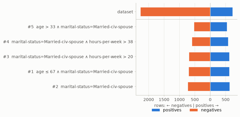
The first row is the dataset. For each subgroup, the bar to the right counts positives and the bar to the left counts negatives. Compare both the total length and the balance; a visually pure but tiny group may have limited scope.
What to remember
The same pattern—fit a target, generate conditions, configure a task, execute a search, inspect the results—works for many target types. The target and quality function express the analysis question. The search algorithm determines how the permitted descriptions are explored.
Experiment. Change MinSizeFilter(100) to MinSizeFilter(1000), then change
depth=2 to depth=1. Which differences are caused by excluding small groups,
and which by excluding combinations? Keep everything else fixed while comparing.