Reading results and choosing visualizations
The highest score is the start of interpretation. A useful report should make clear who belongs, how many rows support the pattern, what differs, and how the selected descriptions relate to one another.
A result table with the right context
from sklearn.datasets import load_iris
import matplotlib.pyplot as plt
import pysubgroup as sd
from pysubgroup import visualization as viz

X, y = load_iris(return_X_y=True, as_frame=True)
data = X.assign(species=y)
target = sd.BinaryTarget().fit(data, "species", 2)
conditions = sd.generate_conditions(X, n_bins=4, numeric_candidates="thresholds")
task = sd.SubgroupDiscoveryTask(data, target, conditions, sd.WRAccQF(),
    depth=2, result_set_size=6, filters=[sd.MinSizeFilter(15)])
results = sd.DFS().execute(task)
sd.to_dataframe(results, data, target,
    statistics=["size", "relative_size", "positives", "target_share", "target_share_complement", "lift"],
measures={"WRAcc": sd.WRAccQF(), "share_difference": sd.LiftQF()})statistics=None gives a target-specific default selection; "all" gives all
available statistics. available_statistics(target) lists the valid names.
Vector-valued statistics expand into columns such as share 0 or mean ....
The quality column records the score supplied with each result pair.
Additional measures are recomputed on these rows and this fitted target.
When evaluating descriptions on different data, pass plain rules or label the
original quality explicitly; otherwise the original discovery score can appear
next to statistics from another dataset.
print(sd.available_statistics(target))
rule = results[0][1]
print(rule)
sd.subgroup_data(rule, data).head()
['size', 'relative_size', 'depth', 'positives', 'target_share', 'target_share_complement', 'lift', 'support', 'recall', 'false_positive_rate', 'leverage', 'odds_ratio', 'conviction']
[petal length (cm) > 4.35 ∧ petal width (cm) > 1.3]
The subgroup-complement difference is often larger than the subgroup-dataset difference because the dataset includes the subgroup. State which comparison the quality function uses.
Match the plot to the question
| Question | Plot |
|---|---|
| How large and enriched is each binary subgroup? | plot_subgroup_bars, plot_spineplot |
| What is the size–quality trade-off? | plot_size_quality |
| How are positives and negatives covered? | plot_roc_space |
| Is the numeric target shifted or spread out? | plot_target_distributions |
| How do descriptors vary within groups? | plot_attribute_distribution |
| Are the results nearly the same rows? | plot_overlap, plot_similarity, plot_similarity_dendrogram |
| Which descriptions specialize others? | plot_specialization_graph |
| How do model relationships differ? | plot_model_scatter |
| Where does classifier ranking deteriorate? | plot_performance_curves |
| How unusual is a validation statistic under its null model? | plot_null_distribution |
These designs connect to the subgroup visualization and descriptive rule-mining literature Kralj et al., 2005Lavrač et al., 2004Duivesteijn et al., 2016.
Size and quality together
fig, axes = plt.subplots(1, 2, figsize=(12, 4))
viz.plot_spineplot(results, data, target, ax=axes[0])
viz.plot_size_quality(results, data, target, ax=axes[1])
fig.tight_layout()
plt.show()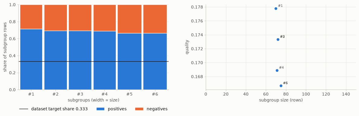
In a spineplot, width represents size and the internal split represents the target share. A size–quality scatter shows whether the ranking is dominated by small extreme groups or larger moderate groups. The panels answer related but different questions.
ROC space for subgroup membership
viz.plot_roc_space(results, data, target, isometrics=sd.WRAccQF())
plt.show()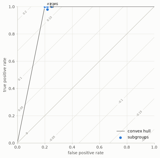
Here a subgroup description acts as a binary test of the target label: membership
means predicted positive. A point gives its false-positive and true-positive
rates. Quality contours show which points score equally under WRAcc. This plot
is not the ROC curve of a soft classifier within a subgroup; that is
plot_performance_curves.
Overlap is part of interpretation
fig, axes = plt.subplots(1, 2, figsize=(12, 4))
viz.plot_overlap(results, data, target, ax=axes[0])
viz.plot_similarity(results, data, ax=axes[1])
fig.tight_layout()
plt.show()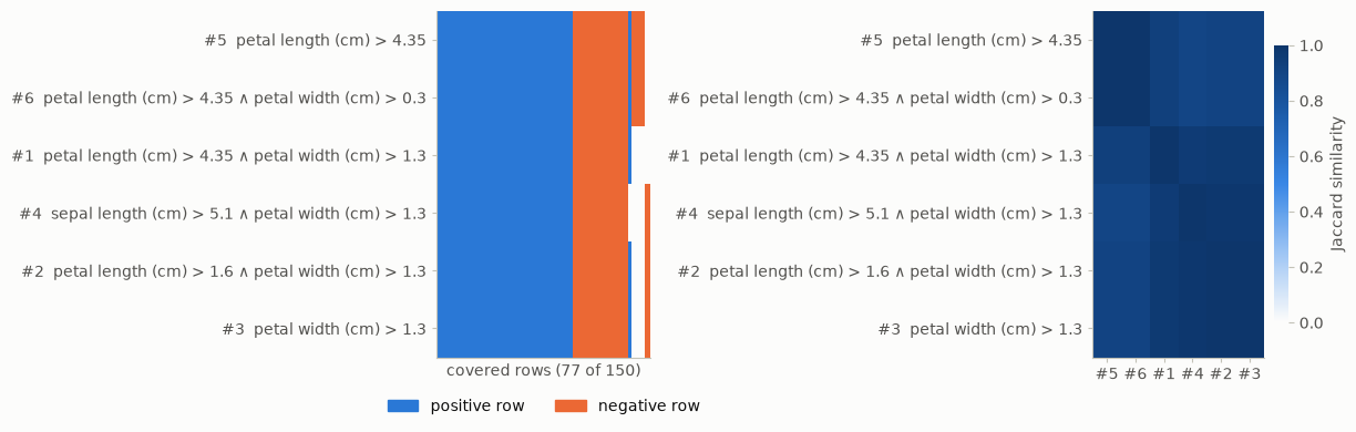
Jaccard similarity compares row sets by intersection divided by union. A block of very similar groups suggests that the ranked list repeats one theme. Do not sum subgroup sizes to estimate the number of distinct covered people.
masks = sd.utils.subgroup_masks(results, data)
print("Sum of subgroup sizes:", masks.sum())
print("Distinct covered rows:", masks.any(axis=0).sum())
Sum of subgroup sizes: 435
Distinct covered rows: 77
From output to a report
For each selected result, report the description, count, target effect in interpretable units, comparison population, and discovery/validation status. Record the search space, quality measure, constraints, and algorithm so that the process can be reproduced. A chart without these details can conceal a different question than the reader assumes.
All plotting functions accept ax= and theme="light" or "dark", and return
a matplotlib Axes. Similarity plots need only results and data; plots of
target statistics also take the target. For presentation-quality figures, select a small result
set and choose a figure size that keeps descriptions readable.
Experiment. Select the five best scores and then select five low-overlap results from a larger candidate list. Which plot best communicates the change?
- Kralj, P., Lavrač, N., & Zupan, B. (2005). Subgroup Visualization. SiKDD. https://aile3.ijs.si/dunja/SiKDD2005/Papers/KraljSubgroupVizualizationSiKDD2005.pdf
- Lavrač, N., Kavšek, B., Flach, P., & Todorovski, L. (2004). Subgroup Discovery with CN2-SD. Journal of Machine Learning Research, 5, 153–188. https://jmlr.org/papers/v5/lavrac04a.html
- Duivesteijn, W., Feelders, A. J., & Knobbe, A. (2016). Exceptional Model Mining: Supervised Descriptive Local Pattern Mining with Complex Target Concepts. Data Mining and Knowledge Discovery, 30, 47–98.